The Weekly Update

As of the Friday’s close, the Nasdaq and the Emerging Markets gave a buy signal. Looks like the noise around the Japan debacle, Libya and whatever else has settled, and the markets have resumed into the direction of least resistance.

Asset	Symbol	Position	Date In	Gain
S&P 500	^GSPC	Long	2010-09-30	15.12%
US REIT	VNQ	Long	2010-07-23	14.16%
Nasdaq 100	^NDX	Long	2011-03-25	0%
Emerging Markets	EEM	Long	2011-03-25	0%

The Weekly Update

(Finally) A few changes in the positions. As of last Friday, both the Nasdaq 100 and the Emerging Markets closed below their 20-week moving average which constitutes closing these positions.

Asset	Symbol	Position	Date In	Gain
US REIT	VNQ	Long	2010-07-23	14.38%
S&P 500	^GSPC	Long	2010-09-30	12.09%

The US REIT position is still open. So is the S&P 500 position, however, it is based on a 10-month moving average, thus, it is updated only at the end of the month. It is worth noting however that it is more than 6% above it’s monthly moving average, so unless something drastic happens it seems likely it will be intact by the end of the month.

The Nasdaq 100 position was opened on September 3th, 2010 and it delivered 18.75% gain. If the double ETF, QLD, was used instead, the gains would have been boosted to 39.23%! I am not recommending using double ETFs, only trying to make the point that double ETFs are an easy and reliable way to leverage when combined together with trend-following strategies, which goes against the “common” knowledge.

The Emerging Markets position was the third whipsaw leading to a loss lately. Here is the list of the last five trades:

Date In	Price In	Date Out	Price Out	Gain	3x Gain
2010-07-23	39.97	2011-01-28	45.33	10.16%	27.79%
2011-02-04	46.50	2011-02-11	45.63	-1.87%	-5.84%
2011-02-18	46.31	2011-02-25	45.52	-1.71%	-5.45%
2011-03-04	46.90	2011-03-18	45.23	-3.56%	-11.02%

This sequence of trades is quite illustrative of the trend-following results. A few trades are successful, the hope is that the successful trades will deliver gains large enough to cover for the losing trades plus some more. In the EEM case, the last three losing trades have left only 2.47% from the last gain. Even more stunning is that using a 3x ETF, after the last trade, the previous 27.79% gain is reduced to a mere 1.2%! That’s why it’s important IMO to do these analysis.

Reducing the whipsaws is essential, but certainly non-trivial. In my opinion, that’s the place to spend efforts improving these systems.

Trading at the Close

A newer, extended version of this post can be found on my new blog.

For back-testing, the typical approach is to use daily closing prices both for the signal and for the entry point. Implementing such a system in practice however is not straightforward. The most obvious problem is that the close remains unknown until the end of the day, thus, we don’t know what our action needs to be before the very end of the trading day.

The way I approach this problem usually is by computing the actions for all possible scenarios. Sometimes that’s easy. For example in this earlier article I have shown how to pre-compute the EMA which would trigger a change in the position. Although it looks great in theory there are two problems with this approach:

It works mostly for simple models (consider reversing the stochastic indicator)
The implementation would require different code (from what we have already written for the back testing), so bugs are likely

Even if the second bullet doesn’t apply to you (I keep hearing there are some bright individuals who write error free code), one still has to deal with the first, so bear with me. We need an alternative.

The simplest solution is to use brute force. It all depends on the strategy, but in general the idea is to first generate the set of possible outcomes (for example all possible closing prices for the next day), then to attach each possible outcome to the end of the series, then run the engine generating the signals (from the back testing code base) on each of these possible series and keep the results.

Let’s consider for example contrarian trading of SPY (S&P 500) using RSI(2). It is unlikely that the SPY will move more than 5% either way on any single day. Thus, using the last day close we can generate all closing prices (rounding to a penny) for the next day within 5% of the today’s price. For each of these prices we compute RSI(2) and the corresponding position.

Finally we need to execute the indicated trade. Either use a broker who allows limit order at the close, like Interactive Brokers. Or, pick a random time between 3:30 and 4:00 on the next day, connect at that time, look at the price and manually execute the pre-determined action for this price.

The added benefit of this approach is that it does not require much new code – the new code is to generate the list of possible outcomes, for the rest we execute the same code we used in the back testing.

How realistic is this in real life? Works quite well IMO. For instruments which are traded very actively, it should be random whether a few points are made or lost compared to the back tested on-close trading. For instruments that are not traded too actively, putting a limit order a penny above the “last price” typically does not result in a slippage of more than 2 pennies, which can easily be factored into the model. Of course, it misses some trades (think wide spreads). In all these discussions, I am mostly concerned of highly liquid ETFs – certainly one cannot use this strategy for penny stocks. If intra-day data is available, the slippage can even be modeled nicely using historic intra-day data.

The Weekly Update

Considering what’s happening around the globe, the markets seem to be holding quite well. A little pullback, but still long on all major indexes. With the exception of S&P 500, everything else is getting pretty close (within 5%) to their moving average – finally some excitement after this long lasting trend.

Asset	Symbol	Position	Date In	Gain
Nasdaq 100	^NDX	Long	2010-09-03	22.93%
US REIT	VNQ	Long	2010-07-23	15.82%
S&P 500	^GSPC	Long	2010-09-30	14.29%
Emerging Markets	EEM	Long	2011-03-04	-1.86%

 

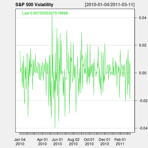
Volatility has also been picking up lately, but nothing out of the ordinary so far:

library( quantmod )
getSymbols( "^GSPC", from="1900-01-01" )
GSPC.rets = diff( log( Cl( GSPC ) ) )
index( GSPC.rets ) = as.Date( index( GSPC.rets ) )
lineChart( theme="white", GSPC.rets["2010/"], name="S&P 500 Volatility" )

 

S&P 500 Volatility

Investing with the Odds

In this previous post, I showed that a look at the correlations in the daily returns of S&P 500 should have lead to a very profitable investing strategy. I also promised to show the results of this strategy in the 80s, but I am not going to do that, because MarketSci has done so in several posts already.

Instead, let’s try to find a more recent “arbitrage” situation like that. Looking into more recent history, and using 126 (half a year) days to compute the autocorrelation function, I got back to August the 30th, 2007:

S&P 500 ACF on August 29 and 30, 2007

As the graph illustrates, the correlation moved into significant territory at the close of August 30. There is a significant negative correlation in the first lag. Looking at this chart, our strategy should be “go short at the close of a positive day, go long at the close of a negative day”. This situation (strong correlation in the first lag) seemed to last until February the 2nd, 2008. Computing the returns (some of the code was borrowed from an article on FOSS Trading, code at the end) we get the following equity chart:

Equity Growth August 30, 2007 - February 4, 2008

How do we know to stop trading using this strategy on February 4th? Why, by the ACF graph of course.

Unless I got something wrong looks damn impressive!

Note, that this is not a trading system, it is just an attempt to approach markets in a much more scientific and systemic way.

Finally the R code:

getSymbols("^GSPC", from="2005-01-01")
GSPC.diffs = diff( Cl( GSPC ) )
GSPC.up = lag( ifelse( GSPC.diffs > 0, -1, 0 ), 1 )
GSPC.down = lag( ifelse( GSPC.diffs < 0, 1, 0 ), 1 )
GSPC.both = GSPC.up + GSPC.down
GSPC.ret = ROC(Cl(GSPC), 1)
GSPC.eq = cumprod( 1 + GSPC.both["2007-08-30/2008-02-04"]*GSPC.ret["2007-08-30/2008-02-04"] )
plot( GSPC.eq, main="Equity Growth Aug 30, 2007 - Feb 04, 2008" )