More orthodox ARMA/GARCH trading

The system described in the earlier series for ARMA trading was in fact an “extreme” version of the more common, orthodox approach prevailing in the literature. Recently I tried using R to reproduce the results of a particular paper, and that lead to a lot of new developments …

How is typically ARMA trading simulated? The data is split into two sets. The first set is used for model estimation, an in-sample testing. Once the model parameters are determined, the model performance is tested and evaluated using the second set, the out-of-sample forecasting. The first set is usually a few times larger than the second and spans four or more years of data (1000+ trading days).

I wanted to be able to repeat the first step once in a while (weekly, monthly, etc) and to use the determined parameters for forecasts until the next calibration. Now, it’s easier to see why I classified my earlier approach as an “extreme” – it does the model re-evaluation on a daily basis. In any case, I wanted to build a framework to test the more orthodox approach.

To test such an approach, I needed to perform а “rolling” forecast (have mercy if that’s not the right term). Let’s assume we use weekly model calibration. Each Friday (or whatever the last day of the week is) we find the best model according to some criteria. At this point we can forecast one day ahead entirely based on previous data. Once the data for Monday arrives, we can forecast Tuesday, again entirely based on previous data, etc.

My problem was that the package I am using, fGarch, doesn’t support rolling forecasts. So before attempting to implement this functionality, I decided to look around for other packages (thanks god I didn’t jump to coding).

At first, my search led me to the forecast package. I was encouraged – it has exactly the forecast function I needed (in fact, it helped me figure out exactly what I need;)). The only problem – it supports only mean models, ARFIMA, no GARCH.

Next I found the gem – the rugarch package. Not only it implements a few different GARCH models, but it also supports ARFIMA mean models! I found the documentation and examples quite easy to follow too, not to mention that there is an additional introduction. All in all – a superb job!

Needless to say this finding left me feeling like a fat kid in a candy store (R is simply amazing in this regard!). Most likely you will be hearing about mew tests soon, meanwhile let’s finish the post with a short illustration of the rugarch package (single in-sample model training with out-of-sample forecast):

library(quantmod)
library(rugarch)

getSymbols("SPY", from="1900-01-01")
spyRets = na.trim( ROC( Cl( SPY ) ) )

# Train over 2000-2004, forecast 2005
ss = spyRets["2000/2005"]
outOfSample = NROW(ss["2005"])

spec = ugarchspec(
            variance.model=list(garchOrder=c(1,1)),
            mean.model=list(armaOrder=c(4,5), include.mean=T),
            distribution.model="sged")
fit = ugarchfit(spec=spec, data=ss, out.sample=outOfSample)
fore = ugarchforecast(fit, n.ahead=1, n.roll=outOfSample)

# Build some sort of indicator base on the forecasts
ind = xts(head(as.array(fore)[,2,],-1), order.by=index(ss["2005"]))
ind = ifelse(ind < 0, -1, 1)

# Compute the performance
mm = merge( ss["2005"], ind, all=F )
tail(cumprod(mm[,1]*mm[,2]+1))

# Output (last line): 2005-12-30  1.129232

Hats down to brilliancy!

ARMA Models for Trading, Part VI

All posts in this series were combined into a single, extended tutorial and posted on my new blog.

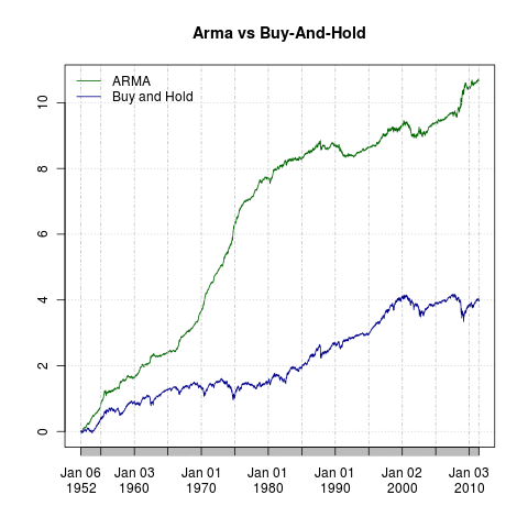
In the fourth posting in this series, we saw the performance comparison between the ARMA strategy and buy-and-hold over the last approximately 10 years. Over the last few weeks (it does take time, believe me) I back-tested the ARMA strategy over the full 60 years (since 1950) of S&P 500 historic data. Let’s take a look at the full results.

ARMA vs Buy-and-Hold

It looks quite good to me. In fact, it looks so impressive that I have been looking for bugs in the code since. 🙂 Even on a logarithmic chart the performance of this method is stunning. Moreover, the ARMA strategy achieves this performance with a maximum drawdown of only 41.18% vs 56.78% for the S&P 500. Computing the S&P 500 returns and drawdowns is simple:

library(quantmod)
library(timeSeries)

getSymbols("^GSPC", from="1900-01-01")
gspcRets = Ad(GSPC) / lag(Ad(GSPC)) - 1
gspcRets[as.character(head(index(Ad(GSPC)),1))] = 0
gspcBHGrowth = cumprod( 1 + gspcRets )
head(drawdownsStats(as.timeSeries(gspcRets)),10)

The above code will produce the 10 biggest drawdowns in the return series. To compute the ARMA strategy growth, we first need the daily indicator. This indicator is what took so long to compute. It is in Excel format (since WordPress doesn’t allow csv files). To use the file in R, save it as csv, without any quotes, and then import it in R via:

library(quantmod)
gspcArmaInd = as.xts( read.zoo(file="gspc.all.csv", format="%Y-%m-%d", header=T, sep=",") )

The first column is the date, the second the position for this day: 1 for long, -1 for short, 0 for none. Note, the position is already aligned with the day of the return (it is computed at the close of the previous day), in other words, no need to shift right via lag. The indicator needs to be multiplied with the S&P 500 daily returns, and then we can follow the above path. The next two columns are the number of auto regressive and the number of moving average coefficients for the model giving the best fit and used for the prediction. The GARCH components are always (1,1).

The only thing I didn’t like was the number of trades, a bit high for my taste – 6,346, or a trade every 2.35 days on average. This has the potential to eat most of the profits, more so in the past than today, however (lower transaction costs, higher liquidity). Still, taking into account the gains from this strategy together with the exceptional liquidity of S&P 500 instruments (SPY for instance trades about 167.7 million shares lately), should suffice to keep a significant amount of the profits.

Last, the simple R-code that produced this nice chart from the two growth vectors is worth showing:

png(width=480, height=480, filename="~/ttt/growth.png")
plot(log(gspcArmaGrowth), col="darkgreen", main="Arma vs Buy-And-Hold")
lines(log(gspcBHGrowth), col="darkblue")
legend(x="topleft", legend=c("ARMA", "Buy and Hold"), col=c("darkgreen", "darkblue"), lty=c(1,1), bty="n")
dev.off()

Pretty neat if you ask me! Code snippets like this one are what makes me believe command line interface is the most powerful interface.

ARMA Models for Trading, Part V

All posts in this series were combined into a single, extended tutorial and posted on my new blog.

Once back testing is done and the results of the trading system are convincingly positive, it’s time to move it to production. Now, how do we implement something like the ARMA techniques I described earlier in practice (assuming a retail brokerage account)?

In an earlier post I discussed the problems related to trading at the close and various solutions. Thus, in this post, I will discuss only the two obstacles I had to overcome for the ARMA methods.

My implementation was to compute a table of actions for each instrument I am interested in. Here is an example:

-0.99%, 1
-0.98%, 1
-0.97%, 1
-0.96%, 1
-0.95%, -1
-0.94%, -1
-0.93%, -1
-0.92%, -1
-0.91%, -1
-0.9%, -1

The above table tells me what position I am supposed to take at the close of the day for various changes (as a percentage) in the price. In the above example, anything up to and including -0.96% is a long position. In other words, if the instrument loses more than -0.96% – take long.

The first problem I found was the computational time. These computations are expensive! I had two choices – code everything in C or buy hardware. Obviously I went after the latter solution – no idea how long it would have taken to port everything successfully to C. For less than $900 I managed to assemble an i7 system which was running a few orders of magnitude faster than my laptop. Moreover it is able to run up to 8 workloads in parallel. If you are unfamiliar, i7 has four cores plus hyper-threading, which makes it sort of similar to an eight core machine and so far it has proved good enough to compute 4 to 5 maps in about 3 hours. All the computations are run in parallel as daily cron jobs in Linux. The results are sent to me in an email. 🙂 The scripts implementing the infrastructure are available on the quantscript project.

The bigger problem was that quite often the computations were not stable enough. In the above example there was a single switch between the long and the short position (at -0.95%). Thus, at 15:55, if the instrument is away from this point, one can take the position with confidence that it won’t cross the line in the last second. Of course, it’s not going to be perfectly on the close, but on average, you shouldn’t expect high negative impact from this type of slippage. Same holds if one is trading moving averages – there is a single prices that separates the long and short position and it can be even determined mathematically.

No such luck for my ARMA implementation, quite often the table of actions looks like:

0.75%, 1
0.76%, 1
0.77%, -1
0.78%, 1
0.79%, 1
0.8%, -1
0.81%, -1
0.82%, 1
0.83%, 1
0.84%, 1
0.85%, -1

If the price is within this range in the last few minutes, there is no guarantee whether it will stop on a long or on a short. So what to do? My solution was simply to not take a position if the price is within an unstable region nearby the close. The alternative is to take the position and be happy with it until at least the open on the next day. After the close we can compute the exact position and if we did the wrong thing, bought when we were supposed to sell, we can close the position at the next day open. Sometimes we will get lucky and it will move in the directions that benefits us regardless of what the system says.

This brings me to the last point – after the close is known, I compute the precise positions and check against the actual positions. If necessary I might take corrective actions during the next day.

My experience so far from a trading point of view is quite positive. What I described above is not too hard to follow in practice. I hope it proves worth the efforts. 😀

ARMA Models for Trading, Part IV

All posts in this series were combined into a single, extended tutorial and posted on my new blog.

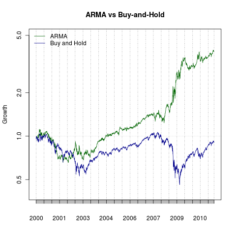
The last post promised to show some back testing results for the ARMA techniques. I decided to use the S&P 500 index for this purpose.

ARMA vs Buy and Hold

What really impresses me in the above char it the staggering performance of this approach during the financial crisis. As if it was feeding on the increased market volatility! This fact is also illustrated by the side by side annual comparisons, which I usually use to get an idea of the long term performance.

Year	ARMA	Buy and Hold
2001	-25.80%	-13.04%
2002	7.14%	-23.37%
2003	28.04%	26.38%
2004	13.66%	8.99%
2005	8.59%	3.00%
2006	17.26%	13.62%
2007	1.85%	3.53%
2008	100.96%	-38.49%
2009	9.75%	23.45
2010	16.82%	12.78

Both systems performed similarly during the 2000/2002 recession, however, there is a stark difference in the performance during the 2008/2009 crisis. While buy and hold was losing money, the ARMA method registered it’s best year ever.

Let’s close with the answers to some obvious questions:

Why did I show only the performance of the last 10 years?
Believe it or not this is a very expensive computation. In fact, I have assembled a powerful i7 CPU machine just to be able to back test and trade these models. Almost 2 full days were necessary to compute the ARMA index for the past 10 years! I will consider publishing back testing for previous years, however, since S&P 500 is not a primary instrument for my trading, that’s not too likely to happen.

What parameters I used to compute the ARMA index?
The code is close to the code I have published in previous posts. I have used the fGarch package and my code always picked a GARCH(1,1) model. For the ARMA part, my code used all models between (0,0,1,1) and (5,5,1,1). I used 500 days of history. I mostly used the skewed Generalized Normal Distribution, specified by the cond.dist=”sged” parameter of garchFit, however, I obtained similar results using cond.dist=”sstd”.

It has become a lengthy and time-consuming post, so I will stop here. If I ever decide to do another post on this topic – I would likely discuss the obstacles I encountered while trading these models on a daily basis …

ARMA Models for Trading, Part III

All posts in this series were combined into a single, extended tutorial and posted on my new blog.

In the last post I showed how to pick the parameters for the ARMA model. The next step is to determine the position at the close. One way to do that is by a one day ahead prediction, if the prediction comes negative (remember the series we are operating on is the daily returns) then the desired position is short, otherwise it’s long.

library(quantmod)
library(fArma)

getSymbols("SPY", from="1900-01-01")
SPY.rets = diff(log(Ad(SPY)))
SPY.arma = armaFit(~arma(0, 2), data=as.ts(tail(SPY.rets,500)))
predict(SPY.arma, n.ahead=1, doplot=F)

Now, to build an indicator for back testing, one can walk the daily return series and at each point perform the steps we covered so far. The main loop looks like (in pseudocode):

for(ii in history:length(dailyRetSeries))
{
   tt = as.ts(tail(head(dailyRetSeries, ii), history))
   ttArma = findBestArma()
   predict(ttArma, n.ahead=1, doplot=F)
}

Where history is the look-back period to consider at each point, I usually use 500, which is about two years of data. Although the above code is simply an illustration, I hope the main idea is pretty clear by now.

As mentioned earlier, findBestArma needs to be surrounded by a tryCatch block. Same goes for the predict – it may fail to converge. What I do is to have predict included in findBestArma, ignoring models for which the prediction fails.

Another improvement is to use ARMA together with GARCH. The latter is a powerful method to model the clustered volatility typically found in financial series. Sounds complex, but it turns out to be pretty straightforward in R. Just to give you an idea:

library(quantmod)
library(fGarch)

getSymbols("SPY", from="1900-01-01")
SPY.rets = diff(log(Ad(SPY)))
SPY.garch = garchFit(~arma(0, 2) + garch(1, 1), data=as.ts(tail(SPY.rets, 500)))
predict(SPY.garch, n.ahead=1, doplot=F)

That’s all I have to say on the theoretical side. I will finish this series with more implementation details and some back testing results in the next post …

ARMA Models for Trading, Part II

All posts in this series were combined into a single, extended tutorial and posted on my new blog.

We left the last post at the point of determining the best ARMA model. Before continuing the discussion, however, I would like to make a few points that might seem a bit questionable or unclear:

• We model the daily returns instead of the prices. There are multiples reasons: this way financial series usually become stationary, we need some way to “normalize” a series, etc
• We use the diff and log function to compute the daily returns instead of percentages. Not only this is a standard practice in statistics, but it also provides a damn good approximation

Now back to choosing the best fitting ARMA model. A well known statistic to measure the goodness of fit test is AIC (for Akaike Information Criteria). Once the fitting is done, the value of the aic statistics is accessible via:

xxArma = armaFit( xx ~ arma( 5, 1 ), data=xx )
xxArma@fit$aic

There are other statistics of course, which for instance penalize models with mode parameters to avoid over-parametrization, however, typically the results are quite similar.

To summarize, all we need is a loop to go through all parameter combinations we deem reasonable, for instance from 0 to 5, inclusive, both for the AR (the first component) and the MA (the second component), for each parameter pair fit the model, and finally pick the model with the lowest AIC or some other statistic. The full code for findBestArma is at the end of the post.

In the code below, note that sometimes armaFit fails to find a fit and returns an error, thus quitting the loop immediately. findBestArma handles this problem by using the tryCatch function to catch any error or warning and return a logical value (FALSE) instead of interrupting everything and exiting with an error. Thus we can distinguish an erroneous and normal function return just by checking the type of the result. A bit messy probably, but it works.

findBestArma = function( xx, minOrder=c(0,0), maxOrder=c(5,5), trace=FALSE )
{
   bestAic = 1e9 
   len = NROW( xx )
   for( p in minOrder[1]:maxOrder[1] ) for( q in minOrder[2]:maxOrder[2] )
   {   
      if( p == 0 && q == 0 ) 
      {   
         next
      }   

      formula = as.formula( paste( sep="", "xx ~ arma(", p, ",", q, ")" ) ) 

      fit = tryCatch( armaFit( formula, data=xx ),
                      error=function( err ) FALSE,
                      warning=function( warn ) FALSE )
      if( !is.logical( fit ) ) 
      {   
         fitAic = fit@fit$aic
         if( fitAic < bestAic )
         {   
            bestAic = fitAic
            bestFit = fit 
            bestModel = c( p, q ) 
         }   

         if( trace )
         {   
            ss = paste( sep="", "(", p, ",", q, "): AIC = ", fitAic )
            print( ss )
         }   
      }   
      else
      {   
         if( trace )
         {   
            ss = paste( sep="", "(", p, ",", q, "): None" )
            print( ss )
         }   
      }   
   }   

   if( bestAic < 1e9 )
   {   
      return( list( aic=bestAic, fit=bestFit, model=bestModel ) ) 
   }   

   return( FALSE )
}

ARMA Models for Trading, Part I

All posts in this series were combined into a single, extended tutorial and posted on my new blog.

Lately I have been testing trading models based on methods from various fields: statistics, machine learning, wavelet analysis and others. And I have been doing all that in R! In this series, I will try to share some of these efforts starting with the well-known from statistics Autoregressive Moving Average Model (ARMA). There is a lot of written about these models, however, I strongly recommend Introductory Time Series with R, which I find is a perfect combination between light theoretical background and practical implementations in R.

In R, I am using the fArma package, which is a nice wrapper with extended functionality around the arima function from the stats package (used in the book). Here is a simple session of fitting an ARMA model to the S&P 500 daily returns:

library(quantmod)
library(fArma)

# Get S&P 500
getSymbols( "^GSPC", from="2000-01-01" )

# Compute the daily returns
GSPC.rets = diff(log(Cl(GSPC)))

# Use only the last two years of returns
GSPC.tail = as.ts( tail( GSPC.rets, 500 ) )

# Fit the model
GSPC.arma = armaFit( formula=~arma(2,2), data=GSPC.tail )


The first obstacle is to select the model parameters. In the case of ARMA, there are two parameters. In other words, there is an infinite number of choices: (0,1), (1,0), (1,1), (2,1), etc. How do we know what parameters to use?

A naive approach would be to back-test strategies with all different combinations over a period of time and pick the best. This is something I have dubbed “hyper system” (ie a system of systems) and can be applied to any combination of indicators and comparative function.

Fortunately there are more robust statistical methods to do that. More on that in the next post …